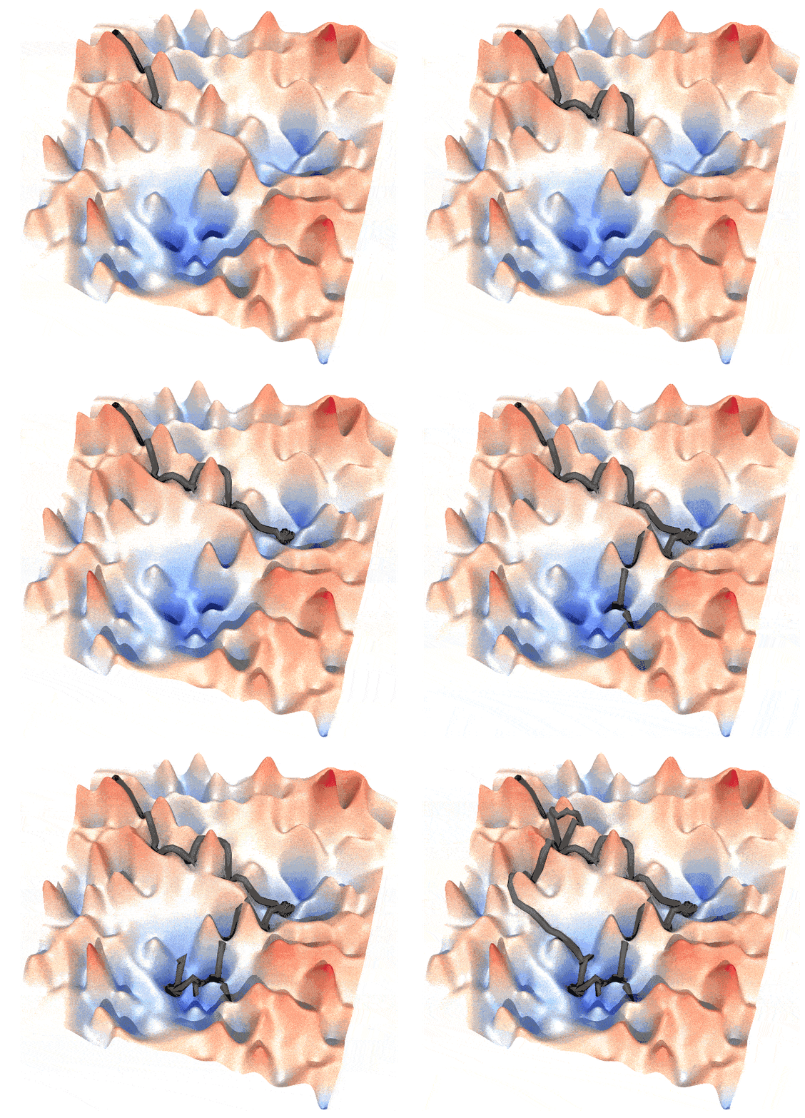
Draw paths on energy landscape

A path on energy landscape is like:

pathway on energy landscape

and this post is a guide to generate such animations.

Step 1: Generate the Energy Landscape

An energy landscape is essentially an energy function $U(\mathbf{x})$. This function can be created in various ways. For example, you might generate a series of Gaussian functions with random parameters $\mu_i$, $\sigma_i$, and weight factors $\omega_i$. From these, you can construct a probability function $P(\mathbf{x}) = \sum_{i=1}^N \omega_i G(\mathbf{x}; \mu_i, \sigma_i)$. The energy function $U(\mathbf{x})$ is then derived using Boltzmann inversion: $U = -k_B T \log P$ .

In the example above, I generated a series of Mexican hat functions with varying parameters ($a$), ($b$), and locations.

Step 2: Generate the Path

A path is determined by the dynamics of the system, such as $\dot{\mathbf{x}} = -\nabla U(\mathbf{x})$ or $\ddot{\mathbf{x}} – \dot{\mathbf{x}} = -\nabla U(\mathbf{x})$. By integrating from a starting point, you can generate a path. In our example, the walker follows a cyclic path, which requires an understanding of the Lagrangian.

A walker on an energy surface from point $A$ to $B$ takes the “canonical path” where the Lagrangian is minimized. The probability of the walker being at $A$ at time $t_0$ and reaching $B$ at time $t_1$ is given by:

$$
P(\mathbf{x}_A, t_0 \mid \mathbf{x}_B, t_1) = \frac{1}{Z} \int_{\mathbf{x}(t_0) = \mathbf{x}_A}^{\mathbf{x}(t_1) = \mathbf{x}_B} \mathcal{D}\mathbf{x} \exp\left(-\int_{t_0}^{t_1} L(\mathbf{x}, \dot{\mathbf{x}}, t) \, dt\right)
$$

Maximizing this probability implies minimizing the Lagrangian $L$ (saddle point approximation). Given $L = T – U$ with $T \propto \dot{\mathbf{x}}^2$, we can discretize the integral of $L$ as:

$$
L = \sum_{i=0}^N \lambda_1 (\mathbf{x}_{i+1} – \mathbf{x}_i)^2 – U(\mathbf{x}_i)
$$

where $\mathbf{x}_0 = \mathbf{x}_A$ and $\mathbf{x}_N = \mathbf{x}_B$. Here, $\lambda_1$ is a hyperparameter controlling the path’s tightness. Our goal is to find a series of $\mathbf{x}_i$ that minimizes $L$. This can be achieved using scipy.optimize.minimize

Step 3. Generate the animiation

The output can be drawn by mayavi, in the example I draw the frames of the animation by povray, where .pov files were generated by mayavi. The trajectory is a thick line that slightly shifted higher than the energy landscape surface to ensure a clear view. You can also draw a big point (sphere) at the forefront of a trajectory, to emphasize the walker.

A simple batch GPC-data processing program

To begin with, I must emphasize that this program was not originally deemed necessary. The story dates back to a lab meeting almost six years ago. During the meeting, a student using the GPC instrument complained that the software couldn’t handle batch data processing because it was a “premium” feature, requiring an additional ~$5000 USD fee. After the meeting, I decided to write this program. It includes two main functions: a baseline correction function and a GPC fitting function, which allows data to be further corrected using Mark-Houwink equations. I had forgotten about this program for a long time until recently, when I encountered a peak-finding problem that required baseline correction, and I rediscovered this old program.

import numpy as np
from scipy import signal
from scipy import sparse
from scipy.sparse.linalg import spsolve


# Function for baseline detection using Continuous Wavelet Transform (CWT)
def baseline_cwt_br(t, y, widths=np.arange(1, 61), wavelet=signal.ricker, theta_iter=2, deg=5):
    r'''Automatic baseline detect algorithm via CWT.
    by Carlo G. Bertinetto and Tapani Vuorinen, 2014
    DOI: 10.1366/13-07018, Volume 68, Number 2, 2014. APPLIED SPECTROSCOPY
    '''
    # Compute the Continuous Wavelet Transform (CWT) of the input signal
    cwt_mat = signal.cwt(y, wavelet, widths)

    # Compute entropy for each scale (width) to find the optimal scale
    cwt_mat_p = np.abs(cwt_mat)  # Take absolute value to handle negative peaks
    cwt_mat_n = cwt_mat_p / np.sum(np.abs(cwt_mat_p), axis=1)[:, None]  # Normalize
    H_w = -np.sum(np.nan_to_num(cwt_mat_n * np.nan_to_num(np.log(cwt_mat_n))), axis=1)  # Compute entropy

    # Find the scale (width) with the minimum entropy
    ind_wh = np.argmin(H_w)
    wh = widths[ind_wh]
    cwt_min = cwt_mat[ind_wh]

    # Evaluate threshold using histogram method
    n = 200  # Initial number of bins
    _count = 0
    while _count < theta_iter:
        n_old = n
        p, e = np.histogram(cwt_min, bins=n)  # Compute histogram
        e = e[:-1]
        ind = np.logical_and(p >= p.max() / 3, p <= p.max())
        sigma = (np.sum((e[ind])**2 * p[ind]) / p[ind].sum())**0.5  # Compute standard deviation
        n = int(8 * (cwt_min.max() - cwt_min.min()) / sigma)  # Update number of bins
        if (n - n_old) / n_old < 0.05:
            _count += 1

    # Define baseline indices based on the threshold
    n_ind = np.logical_and(cwt_min > -3 * sigma, cwt_min < 3 * sigma)
    theta = sigma * (0.6 + 10 * cwt_min[n_ind].shape[0] / cwt_min.shape[0])
    baseline_ind = np.logical_and(cwt_min > -theta, cwt_min < theta)

    # Iterative polynomial fitting until convergence
    b_p = y[baseline_ind]
    b_t = t[baseline_ind]
    converge = False
    while not converge:
        n = b_p.shape[0] // 100  # Segment length
        b_p_old = np.copy(b_p)  # Copy previous baseline points
        p = np.polyfit(b_t, b_p, deg=6)  # Fit polynomial of degree 6
        pi = np.poly1d(p)(b_t)  # Evaluate polynomial
        std = np.mean((pi - b_p)**2) ** 0.5  # Compute standard deviation
        ind1 = b_p - pi < 1.5 * std  # Identify points within 1.5 * std
        b_p = b_p[ind1]  # Update baseline points
        b_t = b_t[ind1]
        p = np.polyfit(b_t, b_p, deg=deg)  # Fit polynomial of specified degree
        pi = np.poly1d(p)(t)  # Evaluate polynomial
        ind2 = y - pi < 0  # Identify points below the polynomial
        segs = np.cumsum(np.r_[
            0, np.diff(np.flatnonzero(np.diff(ind2)) + 1, prepend=0, append=ind2.shape[0])
        ])
        for i in range(1, segs.shape[0]):
            seg = ind2[segs[i-1]:segs[i]]
            if seg[0] and (seg.shape[0] >= n):
                b_p = np.append(b_p, y[segs[i-1] + seg.shape[0] // 2])
                b_t = np.append(b_t, t[segs[i-1] + seg.shape[0] // 2])

        # Check for convergence
        if b_p_old.shape[0] == b_p.shape[0]:
            if np.allclose(b_p_old, b_p):
                converge = True

    return p(t)  # Return the computed baseline

This baseline correction algorithm was adapted from a method where the authors used an iterative approach. They fit the baseline, identified from the slow modes of the CWT, with polynomials. In each iteration, outliers are removed until the baseline converges. This method is adequate for signals with high signal-noise ratio, for noisy systems, the signal should be smoothed first.

The second part is the GPC-processing part, the codes are here:

import warnings
import argparse
import numpy as np
import pandas as pd
from scipy.integrate import simps
from scipy.signal import detrend
from matplotlib import pyplot as plt
from scipy import sparse
from scipy.sparse.linalg import spsolve
from baseline import snr
from baseline import baseline_cwt_br
import re


description = """
A simple GPC data analysis program, for
I aint f**king believe that a simple GPC
data analysis program is
worth 30000 RMB aka $5000 USD.
"""

arg_parser = argparse.ArgumentParser(
    description=description, formatter_class=RawTextHelpFormatter)
arg_parser.add_argument('-S', '--standard',
                        dest='standard', type=float, metavar="standard curve",
                        nargs=2, help="Standard curve, slope `k' and intercept `b0'.")
arg_parser.add_argument('-O', '--output',
                        metavar='Output file',
                        default='mwd', dest='out_put',
                        help="Optional, use `mwd' as default prefix.")
arg_parser.add_argument('gpc_file(s)',
                        nargs=+, type=str
                        help='GPC data file(s).')
arg_parser.add_argument('-M', '--method',
                        nargs=+, type=str, dest='method', metavar='Detector(s).',
                        help='GPC detector(s).')
						
						
args = arg_parser.parse_args()
alvars = vars(args)
k, b0 = alvars['standard']
#k, b0 = -0.5005413052736007, 11.278597269990836  # test data.
# TODO: add combination mode of detectors.
detector = alvars['method']
#mark_houwink = pd.read_csv('mh.dat', sep='_')
# MH equation: K_1 M_1^{a_1} = K_2 M_2^{a_2}, universal calibration curve.
# k2, b0_2 = k * (a_2 + 1)/(a_1 + 1), b0 + k * np.log(K_2/K_1)/np.log(10)  # mk equation to transfer M1->M2
# k, b as function of K, a, if we know the k, b0 and K_1, a_1 for a certain polymer.


def std_func(t, k, b0):
    r'''GPC standard curve t->M.'''
    return np.exp((k*t + b0)*np.log(10))


#TODO: add dedrend and find_peak here, or perhaps a GUI?
# RI signal = K_{RI} * dn/dc * c
# LS signal = K_{LS} * (dn/dc)^2 * Mw * c
# Visc. signal = K_{visc} * IntrisicViscosity * c

ret = []
files = alvars['gpc_file(s)']
for i, f in enumerate(files):
	data = np.loadtxt(f)
	t, y = data.T[0], data.T[1]
	while True:
		plt.plot(t, y)
		plt.show()
		s, e = [float(_) for _ in re.split(',\s*|\s+',input("Trim the GPC, start, end: ")) if _ != '']
		inds = np.logical_and(t>s, t<e)
		t1 = t[inds]
		y1 = y[inds]
		plt.plot(t1, y1)
		plt.show()
		if input("End trim? [y|n] ") == 'y':  # trim data
			break
	b = baseline_cwt_br(t1, y1)  # baseline correction
	plt.plot(t1, y1-b)
	plt.show()
	t = t1
	y = y1
	m, i = std_func(t, k, b0), y
	if detector == 'RI':
		p  = i/m * 1/abs(k*np.log(10))  # P(t) -> P(M); the 1/m factor is used to transform P(Log M) -> P(M)
	np.savetxt('%s_%03d.txt' % (alvars['out_put'], i), np.vstack([m, np.abs(p/simps(p, m))]).T, fmt='%.6f')

There are still unresolved “TODO” items, which I hope to complete someday. These may include new functions, such as deconvolution for two-step polymerization.

Learn via using with from ChatGPT

Creating account

To create an account for ChatGPT, please note that it is currently inaccessible in mainland China. Therefore, you will need two tools to register accounts from OpenAI:

  1. Activation SMS: Use sms-activate.org to receive the activation SMS.
  2. Virtual credit card: Obtain a virtual credit card from vvacard.com. It is recommended to use a stable web proxy that matches the geographic information of your proxy with the card’s address.

API proxy

While the web UI of OpenAI is free to use, GPT-4 comes with a $20/month charge. Additionally, using a proxy may result in your account being blocked. To avoid this issue, you can utilize an API proxy. OpenAI recently announced that GPT-4 models are available for paid API accounts, allowing you to pay on demand. We recommend the GitHub project Yidadaa/ChatGPT-Next-Web for a ChatGPT web UI. It supports one-click deployment on Vercel and authentication by setting access codes.

In addition to the web UI service, certain localized projects such as binary-husky/gpt_academic on GitHub require access to the OpenAI API address https://api.openai.com/v1/chat/completions. While the binary-husky/gpt_academic project provides a PROXY option, it is more reliable to deploy a reverse proxy for the OpenAI API address. We recommend the projects gaboolic/cloudflare-reverse-proxy and gaboolic/vercel-reverse-proxy, both of which provide one-click deployment on Vercel/Cloudflare. For personal use, the free plans of Vercel/Cloudflare should suffice. Alternatively, using Nginx on a VPS is also a viable solution.

The final step involves setting up a domain since Vercel’s domains are banned in China.

Although this post is unrelated to the title, I have realized that after using GPT-4 and tools like binary-husky/gpt_academic, I feel that I am no longer necessary. This tool can teach, deduce, perform mathematical calculations, write and debug code, and even write academic papers and respond to reviewers. It is far more capable than me.

*UPDATE* Now Vercel pass the IP address of user to OpenAI so that you have to access Vercel client with valid proxy.

电信IPTV折腾笔记

办电信宽带,加了10块钱/月的iptv,就是折腾的起始。首先强调一下为什么要折腾:电信给的华为悦盒就是一坨狗屎,我本来还是想找个能来回切hdmi的设备,但是华为悦盒实在是太他妈狗屎。最后买了Nvidia Shield Pro,装了Kodi和iptv的插件。

电信鉴权分两个部分,一是IPoE鉴权,具体是option 60即vendor classifier id,与option 12,hostname为盒子的IMEI,就印在盒子后面。二是业务鉴权,用来获取播放列表、电视节目单。

第一部分:option 60与用户名和密码

option 60的内容是用IPoE账户/密码加密生成的,目前解决的方案是将盒子直接连接到电脑,然后抓DHCP的包然后直接复制。不是很懂IPoE的具体原理,不知道这个加密有没有时间戳和过期,至少目前测试是没有,可以复制出来直接用,也可以tcpreplay数据包。

IPoE的用户名和密码对每个电信盒子(同一地区的华为悦盒?)似乎是一样的,具体的用户名和密码去找stbconfig.db,这个需要你能开启adb,或者直接拆盒子提取镜像。没测试给盒子插上优盘然后开debug模式然后读输出的那些txt里有没有,总得来说,这里找到的密码是加密的结果。stbconfig.db里包含用来生成option 60的用户名及密码,以及pppoe的用户名密码,也就是业务账号和密码。stbconfig.db里的密码以加密方式储存,加密方式需要逆向apk,有人逆向出了stbconfig.db里密码的方式:1.用特定字符串(这个种型号、地区的盒子可能不一样,我这里和[1]一样是“IPTV_2012_STB”)的MD5生成AES密钥;2.用(1)的密钥加密密码然后base64一下。解密过程则是先base64 decoding然后用(1)的密钥解密。具体可以看这里

因为第一步的IPoE鉴权可以通过直接抓包盒子完成,似乎没人进一步研究option 60内容的加密算法,我对逆向不是很熟,也有开发环境,信息基本靠自己逐个文件手动点,太麻烦就没进一步尝试。

第二部分:业务鉴权

业务鉴权原则上一定需要业务用户名(UserID)和密码(制作密钥用来生成Authencator),这个在盒子设置里直接读不到,所以要么打电话问10000,要么按照上面的步骤从盒子里提取。根据中国电信iptv技术规范,其业务鉴权分为以下步骤:

  1. 客户端发起登陆请求,通常url带有UserID=xxx&Action=Login
  2. 服务端返回EncryptToken
  3. 客户端向服务器提交Authenticator,EncryptToken,STBVersion,STBID,mac地址,STB鉴权方法(STBType)等
  4. 服务器验证后返回UserToken和鉴权的cookie

UserToken和cookie为鉴权的目标,也是读取频道列表和节目单的凭证。其中STBID,mac地址等信息由盒子决定。比较麻烦的是鉴权方式,这个直接决定怎么去生成Authenticator,版本号包含在STBVersion、STB鉴权方法(STBType)一类的信息里。虽然根据电信的业务标准,这个Authenticator是由

随机8位数+$+EncryptToken+$+UserID+$+STBID+$ip+$+mac+$$CTC

通过3DES加密生成,参数为:ECB PKCS7。但比较麻烦的是加密密钥的生成,这个加密的密钥生成算法应该每个地区的盒子不太一样,需要进一步破解盒子以及逆向各种调用,具体去寻找CTCGetAuthInfo方法,例如[2][3][4],虽然都是由上面的字符串加密,但密码生成的步骤略有不同。虽然麻烦,但还是建议逆向,虽然密钥只有8位,只要不是纯数字,破解起来也是很难的……

但有意思的是,虽然UserToken过期时间很短,但是EncryptToken似乎是长期有效的。而鉴权的原理似乎也是EncryptToken+Authenticator的方式,换句话说,你只要抓取一次EncryptToken和Authenticator,后面能长期使用,这应该算是电信想省事搞出来的?毕竟每次通过步骤(1),都会获取新的EncryptToken,但电信没有加上作废期。我的猜测是,为了省事,每次生成EncryptToken以后,服务端只验证(EncryptToken,Authenticator)对的合法性,并没有校验这个EncryptToken是不是这次生成的,或者校对时间戳。

第三部分:好好搞搞正则表达式,然后在openwrt上serve每次抓来的节目单。

参考:

[1] https://www.znds.com/tv-1165285-1-1.html
[2] https://github.com/dog-god/iptv/blob/master/java/src/com/armite/webkit/plug/Authentication.java
[3] https://github.com/xylophone21/CtcIptvChrome/blob/master/src/ctc_iptv.js
[4] https://github.com/VergilGao/Telecom-IPTV-Mock

TODO:我这里的STBType主要是华为悦盒的型号,所以试试其他地区电信盒子的STB鉴权方式(包括STBVersion,STBType),是不是直接可以通过控制这个变量来选择相应的Authencator生成算法呢?

Rendering molecules with Povray

Povray is a is a high-quality tool to create 3d graphics. Here is my notes on rendering molecules and coarse-grained models.

Ray tracing:

global_settings {
    radiosity {
        count 60
        always_sample on
        recursion_limit 2
        error_bound 0.8
    }
}

Texture:

texture {
    pigment {
        bozo color_map{[-2 rgbt <0.3, 0.3, 0.3, 0.0>][1.0 particleColor]} scale 0.25
    }
    normal { bumps 0.3 noise_generator 2 scale 0.08 }
    finish { specular 0.8 roughness 0.2}
}

Result:

illustration

As marked by blue square, the boto controls the dark spots on the sphere, and bumps creates the look of rolling hills. The specular keyword in a finish statement produces a highlight, which more closely resembles real specular reflection and provides a more credible spreading of the highlights occurring near the object horizons.

Back2Top ^